The real interest rate puzzle, a two-handed case

A nice example of the 'two-handed' aspect of economics is the notion of how a particular variable, say, the real interest rate, will move from the short-run to the long-run. My aim is to try to be able to interpret the movement of this variable across time, and the forces that determine it.

Reason to increase:

The under-investment in a recession will result in a shortage of capital stock to replace depreciation of capital. This shortage of capital stock will translate into negative and reducing inventory levels, which signal to producers to increase investment and capital stock, leading to increased use of resources and eventually to full employment. It is likely that the shortage of capital will make capital scarce- and thus increase the marginal efficiency/cost of capital. Another way of illustrating this is to shift the investment demand curve to the right; this results in upward pressure on real interest rate as well.

Right now the US is relying on an infinite source of capital inflow to fund its investment-savings shortfall. The escalating US debt may give rise to concerns of the ability of the Government to rein in deficits and reduce debt over time via reduced outlays and increased taxes. The removal of capital inflows can occur as investors lose confidence in US assets, and this capital flight will reduce the supply of capital and raise the real interest rate.

The combined effects of a falling dollar and rising real interest rates are tantamount to disaster, and many of the currency crises in Latin America, the Asian financial crisis, followed this path. To make it worse, nominal interest rates were in fact increased in these countries to maintain capital inflows- which futher worsened the domestic economy- fuelling doubts about the soundness of the economy- leading to more capital flight- forcing further interest rate increases...and this adverse feedback loop continued until the currency plunged and the economy underwent a prolonged recession. Now, this is unlikely to occur in the US, given that the source of capital inflows come from countries that require US demand to drive their export-sectors (China, Japan, for example).

Reason to decrease:

Well, we know that the collapse in risk tolerance has led to a widespread increase in liquidity and risk premia, as lenders have to hedge against the risk of default. The process of deleveraging has led to a widespread fall in asset prices, as expectations of bankruptcy impacts upon the asset values of banks, where people fear the fact that a bank sells assets is due to the fact that they are ‘lemon assets’. Now upon recovery, it is obvious that the healthy flow of credit will result in the reduction in credit spreads, with reduced risk premia.

Given that deflationary expectations are emerging, as unemployment increases past the natural rate and output growth falls below potential, this is increasing current real rates. Over time, as the economy begins to recover, the inflationary expectations will increase, lowering real rates for a given nominal rate.

How to deal with the opposing forces on real interest rates? The transition from short-run to long-run:

Typically real interest rates are lower in recessions and higher in a boom-time. This is because in a boom time there are more investment projects, more investment demand, which tends to put upward pressure on the real rate, as the marginal product of capital increases. The only exception I suppose happens when a systemic banking crisis causes a contraction in credit, and rising liquidity and risk premia on private market assets mitigate the necessary cash flow to keep corporate investment going. This is particularly evident in the following graph, which shows little change in mortgage and business rates despite excessive easing by the Fed:

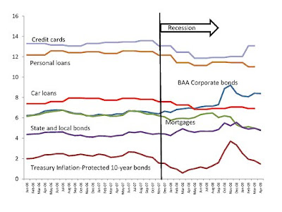
(Graph from Woodward and Hall blog). This clearly shows that at current the credit crunch is leading to a rise in nominal and real interest rates, which are a principal reason for constraining investment and leading to the insufficient demand at present. On the face of this we would expect that real interest rates to lower as the credit crunch abates.

Another aspect is trying to distinguish between real rates and natural real rates persay. For example, at current we suffer from a situation of the real rate being above the natural rate of interest- this correlates to the excess supply of savings as households and firms are deleveraging. There is little doubt that the natural real rate is -ve at the moment, this is the real rate required to restore full employment. Studies conducted by the Fed and Goldman Sachs determine the nominal interest rate required at current is -5/-6%, as determined by a Taylor rule:

(Above graph from Krugman blog, study by Goldman Sachs). There is little doubt that if the natural real rate is seen as -ve at current, then it must move upwards as the economy recovers.

One last point is that, as I have mentioned in previous posts, this crisis is due principally to a global savings glut- which has fed US demand for funds and led to very low interest rates in the US. This was partially due to the fact that investment demand was low following the dot-com bust, and interest rates went to fundamentally unsound levels- fuelling a residential investment boom. Now nominal interest rates remain low, and real rates are likely to remain low once the credit crunch abates- simply because households and firms are in the process of reaching +ve equity, and firms, rather than re-investing cash flow, are likely to use it to pay debt. I predict this insufficient investment will persist until firms and households have delevaraged, and private debt to GDP ratio is more sound. Once physical capital has depreciated and requires replacement, once house prices start trending upwards, it will provide an impetus for physical and residential investment, and increased investment demand for loanable funds will raise real and nominal rates.

Whether this process described above will occur will depend on the persistence of capital inflows into US, which in turn is based on confidence in the $US and whether foreigners believe US debt is guaranteed and will be non-monetised. I believe that the capital inflows into US will reduce over time- as developed countries like China and India open their capital accounts- we should expect higher rate of return in these countries, and a reallocation of capital inflows into these countries. However I doubt that such capital flight from the US will be drastic enough to increase real interest rates in the US, and I do not forsee such a reallocation of capital inflows in the near future.

A great policy lesson from this crisis is that excessively low real rates can cause bubbles. The problem is keeping interest rates low for a prolonged period of time. Unfortunately a big fallback of inflation targeting is that interest rates that are consistent with a stable inflation are inconsistent with asset prices. In the circumstance that asset prices are driven by speculation, then real rates should be increased to curb the increase in asset prices, and ensure they grow at a more sustainable rate. Unfortunately, given underlying inflation is stable, monetary policy becomes insensitive to asset price bubbles- and in the leadup to the housing bubble- the Fed and Treasury encouraged residential investment and ignored the possibility of a house price collapse.

I think the residue from this crisis will result in a more protracted form of lending and securitisation as financial instituions become more risk-averse. This will constrain lending and put further upward pressure on real interest rates. In conclusion, I believe that real interest rates will remain low during the recession (but still above the equilibrium/natural rate of interest), but there are good reasons to believe that real interest rates will rise in the long-run, in the recovery-phase and beyond.

To finish, let me illustrate my short-term/long-term analysis of real interest rates via a graph:

The blue curve is for the natural real interest rate, the black curve for the real interest rate. Note that the period of under-investment corresponds to the period directly after the credit crunch has abated, and is the period of the recession where private sector borrowing is still reducing or below the level required in the recovery phase. I mark the recovery phase as the period in which both the real rate and natural rate of interest are increasing, however the magnitude of this increase is uncertain.

Notice that the reason why the real rate cannot converge to the natural rate during the recession is because of the 0 lower bound on nominal rates! Also, note that I assume that real rate converges to natural rate as economy approaches full employment.

A Chicagoan perspective on fiscal policy

In my blog I have been unrelenting in my factual abuse of extreme right-wing views such as the 'treasury view'. I have never given the chance to present some dignified views of the right. In this post I shall summarise a presentation given by a Chicago University panel featuring Kevin Murhpy, John Huizinga and Robert Lucas. I will be covering Kevin Murhpy's discussion, as that was the most thought-provoking of the three.

Murphy provides a simple model to illustrate how any model that predicts a stimulus to have a multiplier effect depends on certain parameters, and how differing estimates of those parameters drastically change the outcome of whether one is for or against a stimulus. This can be shown as follows:

The parameters are alpha- which measures inefficiency of government (if –ve it implies government is more efficient relative to private sector). Chicago economists typically see alpha as positive, which means that it reduces the nominal measure of government spending. This alpha is effectively a measure of how useful the government purchases and tax cuts are in terms of causing second round and multiple effects of increasing income, and whether a ‘bridge to nowhere’ will actually lead to improved outcomes for society- by raising welfare, rather than just providing an increased measure of GDP. Krugman for example believes the social marginal benefit of increased government purchases exceeds the marginal cost when the economy is below full employment (with the additional constraint of the 0 lower bound preventing a monetary equilibrium from achieving full employment). However conservatives argue that the social benefit is at times unjustified in light of the fact that

i) There are a limited number of ‘shovel ready’ infrastructure projects

ii) There are time lags involved with bidding and organising projects

iii) Some re-allocation of resources is involved in terms of absorbing resources from the private sector.

iv) There is an implicit trade-off between the notion of stimulating the weak parts of the economy- such as Detroit, and the fact that money would be better spent in booming parts of the economy- in which there is inherently higher demand for infrastructure projects.

v) Suppose the projects are aimed at revitalising defunct sectors, such as construction (due to the stock overhang and the severe reduction in demand for housing). It is debateable whether trying to improve the construction industry will pay off in terms of adding to a current excess stock. Re-allocation of workers should occur in a way in which it can be productive for the economy.

vi) In trying to solve v), we could try to re-train construction workers to commit themselves to different activities, for example. Whether this is practical is debateable as trying to reallocate labour is hard to coerce.

These, and many other reasons from the conservative to argue for alpha being positive, and certainly this must be taken into account in terms of assessing the efficacy of the stimulus package.

D is deadweight loss- that is incurred due to the distortions that arise with debt-financed taxes that will be dealt with in the long-term. This goes under the assumption that net present value of taxes are tied to government purchases, implying that taxes need to be raised at some point. Furthermore, Murphy makes the point that the Obama stimulus package seems to consist of tax rebates and transfers in the short-run followed by increases in the marginal rates in the long run. The distortionary effects of taxes, such as the substitution effect, measured by the difference in work effort from a reduction in the marginal income tax rate compared to a tax rebate, show clearly that there are distortions/ deadweight losses incurred from raising marginal tax rates.

F is the fraction of ‘idle resources’ in the economy. Typically, when at full employment, F is 0. However, in these circumstances, with investment below par due to the credit crunch, severely affecting both private sector consumption and investment, with GDP below trend by about 4% and projected at 8% for the end of 2009, F is most likely in close correlation with the business cycle. As mentioned by Murphy, F is also an indicator of the multiplier. If F>1, then the government spending not only uses idle resources, but the rise in income enables the use of more idle resources than intended in the direct effect of increased G. Note that, with accommodative monetary policy (as noted by the fact that any increases in Government financing typically uses the excess loanable funds created by excess supply of money at the above equilibrium interest rate), this means that the crowding out effect is minimal and the level of savings allocated to private sector will change only slightly, if any.

Lamda is the value of idle resources. This is an interesting parameter, as typically one would think that lamda is 0, that any idle resources are of no value. But we know that unwanted inventory accumulation will be written down in value- but it still has value. People not working still value time and are intrinsically worth something…so perhaps there is reason to believe lamda can be positive. Suppose the value of lamda is too high. Would it be more or less encouraging to pro-fiscal stimulus? Interestingly it would mean that the cost of using idle resources increase, and what lamda does is accept the fact that the use of resources, whether private or idle- does incur a cost which must be dealt with in the cost-benefit analysis. And so here it is:


Notice that the first term is the benefit, which is weighed against the 3 costs, the cost of using private resources, the cost of using idle resources, and the deadweight cost. Notice that to put numerical estimates we make G=1, as that way f can be an estimate of the multiplier. Notice that G=1 is required as suppose c is value of private sector resources, then technically the above equation should have (1-f)*c. However, given that we assume the value of private sector resources is equal to value of government spending (with alpha=0), the c is implicitly 1. Thus, we can simplify the inequality to


Now for the fiscal stimulus to have net benefits then it would have to satisfy the above inequality. Now Murphy gives 3 estimates. Let us take team Obama.
Team obama believe that f=1.5, that lamda is 0, alpha is 0 or possibly negative, and d at a conservative estimate of 0.8 (Using Murphy’s neutral estimate from Feldstein’s analysis). The inequality naturally holds as 1.5>0.8. Take Fama’s case. He believes in a complete crowding out effect, and so holds that f=0, and that government spending can only occur in as far as any deadweight loss of future taxes is offset by a relative efficiency of government spending over private sector spending- compensating for future taxes. This may well be the analysis behind government spending during an economic boom. A middle-ground analysis, with conservative estimates of f=0.5, lamda=0.5, means that with d=0.8, government spending needs to be atleast 55% more efficient than private sector spending (ie alpha needs to be less or equal to –0.55). Thus one can see why so many Chicago economists scoff at this Keynesian stimulus package!

Dynamic Scoring: Does the debt burden matter?

The main critique of fiscal policy is the debt burden it places on future generations. It is undoubtedly a huge social cost which does mean the governments of the world need to have a medium and long term fiscal strategy, whereby government expenditures recede, tax revenues increase and the budget moves into surplus. What one must look at is how fiscal stimulus actually reduces the debt burden as it closes the deflationary gap and allows recovery of tax revenue and fiscal retrenchment once the economy is on a self-sustained up swing. This is the concept of dynamic scoring.

Another way to look at dynamic scoring is to note that a particular increase in the deficit of say $X B does not necessarily increase the national debt by $X B in the long run. Deficits lead to increased output and a recovery in taxation revenue as automatic stabilisers kick in. The Keynesian argument expressed in my first post on fiscal stimulus suggests that deficits are ‘self-financing’, in terms of creating a pool of private savings to offset the reduction in government savings. What one must appreciate is how the concept of dynamic scoring has implications for the relative efficacy of government spending and tax cuts.

Krugman illustrates this by back-of-the-envelope calculations, and uses the formula ,

where t is the marginal tax rate. Note that the simple multiplier can be used because interest rates are assumed to be fixed (a fair assumption) With estimates such as MPC=0.5, and t=1/3, we obtain a multiplier of 1/(1-(1/3)) = 1.5. This means for an increase in $100B of government spending, we have an increase of $150B in GDP. From the $150B increase in GDP $50B is collected in taxes (due to t=1/3), and a ‘bang for buck’, that is, the amount of increase in GDP per dollar of the future deficit is 3 (As the future deficit is $50B, and 150/50=3). Thus the recovery of half of the lost revenue comes via increased incomes resulting in increased taxation revenue. It is interesting that dynamic scoring increases the gap between those who prefer infrastructure spending and those who prefer tax cuts. According to tax cuts, the multiplier is , which for MPC=0.5 and t=1/3 is 0.75. Furthermore, given the example of a $100B tax cut, we have an increase in GDP of $75B, and a $25B taxation revenue gain. Thus, the ‘bang for buck’ is only 1, compared to 3 for Government purchases. What this example shows, is that even with a low MPC, Keynesian theory supports deficit spending as the burden on future debt is minimised via taxation revenue recovery from increased incomes.

We have looked at the Keynesian version of dynamic scoring, which claims the ‘bang for buck’ promoting the claim for government spending rather than tax cuts. However, other proponents of dynamic scoring claim that tax cuts are more conducive to growth.

Some aspects of tax cuts being conducive to growth were touched on in my previous post. The central idea of tax cuts is to stimulate investment and increase incentives to work, save and invest, and by changing the relative prices of capital, it encourages a re-allocation into more useful capital. These incentive effects were completely neglected by Krugman’s analysis of ‘bang for buck’ illustrated previously, and it is still open to debate whether tax cuts can lead to greater output effects in the long-term.

A treasury study on the $3 Trillion Bush tax-cuts have found that 20% of the package, which comprised of cuts in capital gains and dividend taxes, led to over half of the economic growth effects. Cash transfers to low-income households, child credits and marriage-penalty relief had negligible incentive effects, and in fact, the treasury predicts higher growth without such tax cuts! Thus it is obvious that the theory of incentive effects of taxes is contingent upon the type of tax. It seems that a consensus on the best incentive effect tax cuts seem to be tax cuts aimed at reducing the cost of capital directly, like capital gains tax, and this is partially because it favours higher-income households. For example, in a survey Stiglitz concludes:

“Pareto efficient taxation requires that the marginal tax rate on the most able individual should be negative…”(Stiglitz)

Thus many believe that marginal tax rate reductions have more incentive and supply-side effects if they are targeted at higher income deciles, contrary to vertical equity and the progressive taxation system.

A more important finding of the treasury report is that the effect of tax cuts is contingent on how it is financed. If it is not financed via immediate reduction in Government spending, than it is assumed in treasury analysis to be financed via an increase in future income taxes. Then we are hit by a deadweight loss of future taxes, as well as Ricardian equivalence measures- of absorbing the tax cuts into increased savings, with no change in consumption, could significantly reduce any demand/output effects. GNP estimates suggest that in the case where tax cuts are financed via reduced G- there is a 0.7% increase. In the case where tax cuts are financed by future increased taxes, there is a 0.9% fall. This disparity reflects the fact that tax cuts cannot be temporary, simply because

i) Temporary tax cuts, if forseen by households, will require them to (in aggregate) purchase government bonds equal in present value to the future tax liabilities from the increased deficit. This will require households to save the full amount of the tax cut, leading to no change in present consumption. This is in perfect ratification with the permanent income hypothesis, which says that consumption trends can only be influenced by permanent changes in income, not temporary changes.

ii) Any reversal of tax cuts will incur a deadweight loss, due to negative incentive effects. In a sense, the tax cut reversal will reverse any growth created by incentive effects, and ruins the dynamic benefits of tax cuts incentivising investment.

Given that tax cuts at present, in Obama’s fiscal stimulus package, are concurrent with even larger government spending increases, this will tend to reduce the effect of tax cuts. This is yet another reason for the Romer-Romer analysis of exogenous tax cuts to fail in light of current circumstances.

It is interesting that the temporary vs permanent concept, a concept outlined in my previous post, provides a powerful argument in favour of government spending. Given that we have proven permanent tax cuts are more effective that temporary tax cuts- simply because it avoids Ricardian equivalence problems, there are numerous problems of maintaining permanent tax cuts, namely, why should we maintain low taxes once the economy returns to normal? Do we permanently cut taxes again once there is another recession? Permanent tax cuts are impractical, temporary tax cuts are ineffective- and given the need to finance the treasury debt via future raised taxes, any dynamic effects of lower taxes will be offset. However, it is possible to make a permanent tax cut work- given that it is financed via a permanent increase in a different tax. Thus Mankiw’s idea of a permanent reduction in payroll tax with a gradual, permanent increase in the gasoline tax is a good idea, with the gasoline tax increasing gradually to enable net output effects from the payroll tax reduction.

Let us examine government spending. If a program requires $100B of government spending each year, consumers may save an amount equal, in present value, to the accumulated deficits, leading to an offsetting reduction in consumption. It is temporary government spending that avoids Ricardian equivalence, as

“…rational households would realise that the increase in their lifetime tax bills would be quite modest, which would imply a small reduction in consumption demand relative to the large increase in government purchases.”(Econospeak)

This shows clearly that there is offsetting consumption, but it is only marginal in light of the fact that the tax burden can be spread across a number of years, thus the offsetting consumption can be spread across a number of years as well. Government must be careful that current projects do not lead to a stream of future projects due to political lobby groups. It is very easy for a temporary increase in Government intervention to become permanent, and this will have disastrous implications for the treasury debt to GDP ratio, which will lead to a more tax-intensive economy in the future.

Dynamic scoring is integral to appreciate the long-term effects of the stimulus package. Through using simple Keynesian analysis, it favours government spending as providing much more ‘bang’ per dollar of future deficit, it is possible that incentive effects of taxes can lead to economic growth, with the increase in GNP leading to a recovery of tax revenue. There are numerous problems with consolidating the incentive effects theory, such as trying to find the relative elasticity of labour demand and supply, to isolate the effect of revenue recovery due to the tax cuts from other variables, the fact that it is contingent upon the type of tax cut- the way the deficit is financed, all of these factors make it very hard to evaluate the dynamic effects of tax cuts. In so far as tax cuts are more easily and readily implemented, they are useful. However, I feel that the first priority is government spending that meets the cost-benefit test, the remainder going towards a well-structured tax cut program, with specific details as to how increased taxes will be implemented in the future without a distortion of the incentive effects created by the tax cuts.

Structure of Fiscal Stimulus: Government Spending or Tax-Cuts?

The multipliers estimated for the Obama plan (Romer and Bernstein) are 1.55 for government purchases and 0.98-99 for tax cuts after 16 quarters (4 years). These are based on simulations done by 2 different agencies; one is the Fed Reserve model, and one from a private forecasting firm. In light of mainstream models- such as Valerie Ramey’s 1.5, it is a ‘fiscal policy’ puzzle as, the head of the National Council of Economic Advisers, Christina Romer, published a recent paper estimating the multiplier for tax cuts at 3.

“tax changes have very large effects on output. Our baseline specification suggests that an exogenous tax increase of one percent of GDP lowers real GDP by roughly three percent. Our many robustness checks for the most part point to a slightly smaller decline, but one that is still well over two percent…”

In the above statement, the ‘exogenous’ in bold is of utmost importance in explaining the reason for why there is such a stark constrast in multipliers. The problem in the model is that the tax cut occurs in a non-systematic, random point, with no reference to the business cycle. This means that

i) we can attribute any output effects solely to the tax cut.

ii) Expectations are more unlikely to adjust, that is, people are unlikely to behave in a ricardian fashion and to save the entire reduction in taxes

The problem of course, is that the current stimulus package can be seen as endogenous, in that it is a direct response to insufficient demand, and is a ‘countercylical’ response. Mankiw explains this as a tax cut designed to offset the demand dampening effects of an event X.

We know that the unfolding of event X on aggregate demand is incomplete, and that any output effects due to the tax cut are likely to be mitigated by the output effect of event X. An event X that comes to mind is the credit crunch, which is leading to a ‘flight to quality’, with excess holdings of money and government debt, and a corresponding rise in precautionary savings. Thus, given that the credit crunch is leading to a rise in the saving rate, it is likely that a tax cut is going to be largely saved (In Macroblog, it notes that the saving rate has gone from –0.1% in 06 to 2.8% in November 08). In any case, the ongoing dampening effects of the financial crisis and the aftermath of current lowering of production in response to lowering demand is likely to offset the direct output effect from the tax cut.

It is interesting to note that in Romer’s paper she makes a reference to tax-based investment incentives,

“For tax-based investment incentives, we used the rule of thumb that the output effects correspond to one-fourth of the effects of an increase in government spending with the same immediate revenue effects. This implies a fairly small effect from a given short-term revenue cost of the incentives. But, because much of the lost revenue is recovered in the long run, it implies a fairly substantial short-run impact for a given long-run revenue loss…"

This makes it clear that Romer believes that dynamic scoring means that ‘bang for buck’, the amount of short-term stimulus added per dollar of debt- is effectively high. In other words, they believe that tax cuts are more effective at recovering revenue in the long-term, and so in light of the effective dollars spent (that is not financed via recovered revenue), the short-run effects seem worthwhile.

By ‘same immediate revenue effects’ I assume that Romer believes that the static deficit increase is the same, whether it be through an increase in G or a reduction in T. Why, according to Romer, would the incentive effects of investment tax-cuts lead to a smaller long-term revenue cost than government spending? In other words, she believes that over time, dynamic estimates of the deficit will be lower for the reduction in T, compared to an equivalent increase in G. This is in stark contrast to Krugman’s estimate in Dynamic Scoring, where he shows clearly that the ‘bang for buck’, the amount of stimulus per dollar of future deficit, is much larger for Government spending than for tax cuts. The difference is of course due to Krugman’s neglect of incentive effects of tax cuts. There is little doubt that investment tax cuts, such as a cut in capital gains tax, company tax, tax rebates for innovation, a cut in payroll tax, do provide some impetus for capital investment, or perhaps greater employment. In fact, Mankiw, in discussion of why the Romers estimate a tax multiplier can reach a maximum of 3, says

“…tax cuts produce a bigger boost in investment demand. This might work through changing relative prices in a direction favourable to capital investment--a mechanism absent in the textbook Keynesian model. Suppose, for example, that tax cuts are not lump-sum but instead take the form of cuts in payroll taxes (as suggested by Bils and Klenow). This tax cut would reduce the cost of labour and, if labour and capital are complements, increase the demand for capital goods. Thus, the tax cut stimulates demand not only by increasing disposable income and consumption spending (the textbook Keynesian channel) but also by incentivizing more investment spending.” (Greg Mankiw)

Mankiw’s opinion of current is to provide a permanent reduction in the payroll tax coupled with a gradual, permanent increase in the gasoline tax. This will equal each other in net present value, so in other words, it ties the budget to be neutral over the course of the business cycle. The idea of payroll taxes, according to Bils and Klenow, has 3 benefits:

1) Like previous stimulus efforts, it has the standard demand side impact (same as cutting checks). But it also stimulates employment directly by reducing the tax penalties for working and for hiring workers. Related, it works under all business cycle models (even including those obeying Ricardian Equivalence).
(2) It targets domestic production better than sending out checks (or a sales tax cut).
(3) It targets lower income households, due to the cap on social security taxes. These households may respond more in both their consumption and employment decisions.

Thus it is obvious that there are many factors behind tax cuts that are not included in simple Keynesian theory. It has supply-side effects, as it targets domestic production via lowering costs of production, and it increases the incentive to raise employment, and capital. Plus, given that payroll taxes are paid by all employers, low and high-income, it will attempt to reduce a proportional tax, thus relieving a greater burden for low-income employers and increasing income equality. Such incentive effects are long-term, and will not really affect the direct 1st round output effects. Given the fact that tax-cuts are more effective in the long-run, and that incentive effects are very hard to analyse using past examples (due to the endogenity problem, that is, it is hard to isolate incentive effects of increased output and revenue recovery from other events).

Thus there is ample reason to believe that tax-cuts are not very stimulating, and in many cases will likely be saved via Ricardian Equivalence measures. In fact, Ricardian Equivalence tends to favour government spending rather than tax cuts, with an emphasis on whether they be temporary or permanent. Though there is no doubt that any tax cut, to have effect, must be permanent, it is impractical to make tax-cuts permanent because, once the economy returns to normal, you cannot renege on the policy and increase those taxes again to be budget neutral. On the other hand, one can argue that Government spending may not be temporary, as many projects may require ongoing funding commitments, and certain political lobby groups may force the Government to continue subsidising their programs. Thus there is a chance that, on either sides of the G vs T debate, there may be a permanent increase in Government involvement, which makes it harder for fiscal policy to be budget neutral in the long-run.

Before I go through a couple more arguments, I would like to surmise my findings above. I have stated that there are real problems in determining multipliers, especially in relation to government spending multipliers vs tax cuts. Simple Keynesian theory is blurred by theories of incentive effects of tax cuts, which tend to arbitarily increase tax multipliers. Thus there are numerous problems in estimating the reaction of households to deficit financed tax cuts/spending increases, and it is this problem of estimation that is causing much angst among economic commentators at present. The only consensus in the multiplier debate is that multipliers are always greater in a less-than full employed economy.

Another argument proposed by Gauti Eggertsson is that tax-cuts may in fact have negative multiplier effects at the 0 lower bound! The reason is simple, Gauti believes that at the 0 lower bound, any supply-side effects will lead to deflationary pressure. This deflationary pressure cannot be counteracted by lower nominal interest rates- as interest rates are fixed at the 0 lower bound. The economy plunges into a deflationary spiral, increasing the output gap, mitigating any output effects from the tax cut. The effect of aggregate supply was covered in my previous post on supply shocks, and I talked about how ‘vice becomes virtue’, that policies to reduce aggregate supply rather than increase it, can be more helpful in preventing a deflationary spiral.

Lastly, I would like to reflect, again, on the endogenity problem of tax cuts. There is an intuitive argument, mentioned previously, that the endogenous event at current is a natural increase in ‘precautionary savings’ and a system-wide deleveraging effect. The need to pay off debt may lead many households to save much of their tax cuts, especially if they believe that the cuts are only a temporary increase in disposable income (thus leading to ricardian effects). This provides an excellent reason for why Romer’s exogenous tax change study lead to a tax multiplier of 3, but the Romer-Bernstein analysis of the Obama package gives a tax multiplier approaching 1. However, Mankiw expresses some distaste for this idea, as he distinguishes between the idea of increases in precuationary savings leading to an increase in the APC (Average propensity to Consume, with differing implications for the MPC (Marginal propensity to consume). Mankiw’s idea stems from his model of the consumption function. His hypothesis is that consumption will be depressed more in lower income groups, a fair assumption as they tend to have larger debt to income ratios, and are at more risk of losing a job (with less insurance as well!).



The above graph is very simplified, but it shows clearly that there is an autonomous fall in consumption, but with an emphasis on lower income groups. Thus, a tax cut, which enables a rise in disposable income, will, on a marginal dollar, be consumed more by a low-income household than a high-income household. This provides a nice rebuttal to the ‘precautionary savings’ fallacy, which implies tax cuts completely ineffective.

There are numerous other arguments which claim that G > T, or T > G, but I can no longer dwell on them here. I tend to favour government spending multipliers being greater, simply because most Macroeconomic models predict this result, and Permanent income, Ricardian Equivalence models predict the same result. I also feel that tax cuts are more effective in a period of full employment, but with under-employment, incentive effects may not have the desired effect, especially due to the fact that investment is constrained in a recession. In fact, I am of the belief that the greater output effects of government spending are more likely to kick-start investment than tax cuts.

Thus fiscal stimulus is necessary…there is no question! But the structure of the fiscal stimulus, whether it is via tax cuts or government spending, is still open to debate. My feeling is that this question will be resolved using this crisis as a precedent, and a consensus will be reached on the efficacy of fiscal and monetary policy in depression-like conditions. No doubt such a consensus will be a hallmark in the history of economic thought, and I for one hope it will bring together a unity resembling the harder sciences.

A supply shock in Depression Economics...how a rise in nominal wages can be stabilising

A few months ago many posts were written, primarily by Krugman, in response to conservatives like Amity Shlaes on the theory of wages in depression economics. In normal times, a rise in nominal wages all round the board is akin to a supply shock, reducing output and raising prices. Such a rise in wages is due to some institutional factor, like Unionisation, or an increase in unemployment benefits or a minimum wage. Or it could be due to an increase in the expected price level, as perhaps firms believe inflation is to rise, and to keep real wages constant, unions demand higher nominal wages.

Using the AD-AS model applied in Fiscal Stimulus part 1, we have

AS: P=P (e)*F (1-Y/L, z)*(1+m)

The AS curve is shifted up by the increase in the expected price level, in the case above. Another case in which it can be shifted is via the cartelising of labour, in which the formation of cartels, or unions, requires controls on wages, in this case, to either be fixed or to grow at a pre-determined rate. Now, the effect on income in the short-run is dependent on the shape of the aggregate demand curve. In normal times, the AD curve is downward sloping (As a reduction in price level raises real money supply, leading to a lowering of the interest rate and increased investment), however, there are reasons to believe the AD curve is vertical or even upward sloping.

i) Given that we are at the 0 lower bound, it means that the real money balance effect has no effect, as increases in real money supply do not translate to lower interest rates. This effect is due to an infinite elasticity of Money demand to the interest rate at the 0 lower bound.

ii) Another determinant of the AD curve is the interest rate sensitivity of investment. The sensitivity of Investment is lower in a recession simply because the variables of confidence and risk play a greater role in determining Investment. This also reduces the effect of price level on AD.

iii) Thirdly, there is the Pigou effect. This looks at the wealth effect of a reduced price level. Krugman makes back-of-the envelope calculations, in which he estimates that with a $800B Monetary Base, and a 20% fall in prices, a wealth effect of 0.05 translates to 800*0.2*0.05=$8 B. Even with a multiplier of 2, the increase in income is $12B, or roughly 0.12% of GDP. If anything the pigou effect is overwhelmed by the Fisher Debt-Deflation effect, where reduced prices increase the real value of debt, and constrain borrowers, and the fact that deflation increases real interest rates and constrains consumption and investment.

The fact that the AD curve is not downward sloping, but rather vertical, has important implications for wages policy. Now the upward shift of the AS curve does not incur a short-run reduction in output.

Thus this model clearly shows that there is no short-run cost in cartelising labour in depression economics.

Now, let us get into this in more detail. First of all, notice the parallel between cartelising labour and the protectionism outlined in my previous topic. The idea of cartelising labour is simply to promote the welfare of those employed, at the cost of others who seek employment but cannot due to labour demand falling in response to higher wages. It is this channel- where rising wages increase unemployment- which is what people like Amity Shlaes argue prolonged the Depression. However, it is clear that protection of Labour has minimal, if any, short-run reduction in Output in a liquidity trap situation.

There are in fact some very stabilising effects of cartelising of labour that may seem hidden. The problem with Shlaes argument is that there is no way a reduction in wages can increase labour demand and can increase employment if it is across the board. If it is concentrated in one particular sector, than we would expect that there is an increase in employment concentrated in that sector. Krugman explains this nicely.

Suppose that wages across the US economy had been, say, 20 percent lower than they actually were. You might be tempted to say that this would make hiring workers more attractive. But to a first approximation, prices would also have been 20 percent lower –so the real wage would not have been reduced. So how would lower wages lead to higher demand for labour? (Krugman)

Thus one must keep in mind that any nominal wage reductions would be in response to deflation, which will essentially maintain real wages, resulting in no AS shifts and no real effect on output. Now, as far as I can tell, cartelising labour has 3 benefits:

i) Firstly, is the fact that cartelising labour can indirectly try to anchor inflationary expectations (as nominal wages usually try to level changes in the expected price level/inflation). Thus it can be an effective policy at getting the economy out of a deflationary trap

ii) Secondly, by being a policy that reduces supply, it brings the economy closer to internal balance. Given that the economy is suffering from insufficient demand, reducing supply via cartelising labour can reduce the output gap.

iii) Thirdly, there are the incentive effects of higher real wages, which, seen as efficiency wages, can try to muster the enthusiasm required for increased work effort. Also, there are significant problems in cutting nominal wages, as it may induce people to leave work as they demand higher wages, or cause unnecessary discomfort or strikes by workers (it may promote worker dislocation, where workers try to move to places offering higher wages or labour cartels). Other supply side effects include reducing worker turnover (As being part of a union requires to remain in the job)

Of the 3 benefits, the first 2 are intrinsically related. Basically, the idea of trying to stabilise prices is useful, as firms set their prices based on labour costs. If labour costs go up, it prevents them from cutting prices- even in light of reducing demand. This prevents a deflationary spiral, and consequently increases the effect of demand-side policies, particularly monetary policy, to achieve internal balance.

There are, however, some problems of cartels (or more generally unionisation). There are long-term costs involved, with Larry Summers, in an academic paper citing that ‘one long-term cause of unemployment is unionisation’. The idea is that unions do increase the natural rate of unemployment, by keeping wage levels up it naturally reduces labour demand. Subsequently it makes it harder for non-union workers to find jobs, as wages tend to be streamlined across union and non-union workers. Also is the fact that given that there is no protection for non-union workers, they are the most likely candidates for lay-offs in light of any constraints a firm faces.

Another problem could be hidden effects on investment demand. Mankiw raises this point by considering what impact the formation of a cartel would have on long-term business investment, which he believes is likely to reduce in light of labour movements. Krugman rebuts this by noting that there was excess capacity and under investment throughout the 1930s (even before labour movements began), and believes that there were more important factors, such as business confidence and profitability, that overwhelmed any labour movement effects. Plus, private investment in fact picked up as Roosevelt went into office, thus further invalidating the idea that the labour movement reduced investment incentives.

There are reasons to favour the claim that unionisation may be a positive move in current circumstances. The ultimate argument is of course whether the short-run benefits of increasing wage growth and hence inflation exceed the long-term costs of unionisation. The key here is whether the increase in Government intervention and initiatives in response to this crisis will recede once we return to normal circumstances, where the private sector is independent and fully de-regulated, and monetary policy returns to being the primary stabiliser. This is a tough question to answer, but as far as I’m concerned, the costs posed by unionisation are minimal and reversible, and is necessary to prevent a deflationary spiral.

Fiscal Stimulus, exchange rates and the temptation of protectionism

Dissecting the protectionism argument

In the planning of Obama’s recovery and re-investment package, there were provisions to purchase ‘only American’ goods and services, such as American steel for construction projects. This ‘only American’ hails memories of protectionist acts such as the Smoot-Hawley tariff of the 1930s that exercised a 30% tariff on all imports to the US. In fact, one of the reasons the Great Depression was prolonged was due to a protectionist stance practised across the world, with trade plummeting, and only returning to pre-crisis levels 20 years later.

The idea of protectionism stems from the idea that imports is a leakage, and that a fiscal stimulus will lose effect if it is contracting foreigners in the projects. The Keynesian ‘complex’ multiplier, with a fixed price level and interest rates, is:
To understand whether protectionism makes sense, we need to look at the Balance of Payments Equilibrium equation, or BP curve. This curve models the pairs of income and interest rates required to fulfil the following condition:

The main problems with understanding open-economy effects are to do more with the capital account effects. Given we are in a liquidity trap (where interest rates have reached the 0 lower bound), we can consider interest rates as rigid. The first implication of rigid interest rates is an invariant capital account, in other words, the saving investment imbalance is rigid. Given the capital account is rigid, the current account must adjust to offset the capital account. What protectionist policies do is to increase the trade surplus/reduce the trade deficit for a given level of exchange rates. This means we have a situation where the BP curve is not in equilibrium. What happens is that the exchange rate adjusts upwards, increasing imports (as they become relatively cheaper) and reducing exports (as they become relatively more expensive) until the current account equals the capital account again. We can model this using the S-I, X-M model, where S-I represents the capital account deficit and X-M represents the current account surplus.
It is important to note that the differential X-M is the same, which means that both the volume of imports and exports has dropped by equivalent amounts. Consequently, protectionism does not achieve its desired goal of achieving greater effects of fiscal stimulus- as the gains of reduced imports come at the expense of reduced exports.

Is fiscal stimulus mitigated by trade flows?

Now we ask ourselves, suppose we do not have the protectionist stance. We now have two problems of the fiscal stimulus.

i) The immediate problem is that any increase in domestic demand from the stimulus will filter through to demand for foreign goods.
ii) Perhaps more importantly, the treasury securities issued by the Government to overseas borrowers strengthens the dollar and leads to a potential crowding out of exports

Both i) and ii) are ways in which fiscal stimulus can cause offsetting trade flows to mitigate the multiplier effect. Nick Rowe provides an explanation for why such an argument does not make sense, and claims that all of the increase in demand will translate to increase in domestic absorption, not increases in demand for foreign goods. In his argument he makes the case for a depreciation of the dollar rather than the appreciation suggested in ii).

Rowe believes that the capital account is fixed, that is, the variables that affect the capital account, namely the domestic and foreign interest rates, are 0, and has the assumption of static expectations, that is, the expected depreciation is 0. This makes sense given the expected depreciation is equal to the interest rate differential, which is assumed constant. Thus any fiscal stimulus will be affected by the BP curve constraint.

CA=Current Account KA=Capital Account
Given that GDP= domestic absorption+Net Exports
Where Net exports=CA, then CA= -KA, which is fixed.

Now the fiscal stimulus will cause income to increase, leading to a deterioration of the current account. Thus, given that the KA is fixed, another variable needs to respond to offset the reduced CA, namely, depreciation of the currency. Thus the increase in imports is offset by depreciation such that X-M stays constant, and we will find that there is effectively 0 crowding out of net exports. Thus Nick Rowe’s analysis shows clearly that, contrary to normal times, a fiscal stimulus can result in depreciation.

Now, his argument is lop-sided, as to have a depreciation of the currency, and yet keep expected depreciation 0 via static exchange rates, doesn’t make sense! Krugman gives a more realistic view, in which he says that short-run changes in trade account may not affect the exchange rate in the long-run. According to his theory, exchange rates stabilise around a long-run exchange rate, where expected depreciation is correlated to the differential between the spot exchange rate and the long-run exchange rate.



Given that i and i* are 0 (in the liquidity trap situation), the exchange rate is dependent on the long-run value. However, it is still possible for short-term changes in the exchange rate to occur due to changes in the trade account. Thus there is a case for Fiscal Policy in the current scenario as trade flows may not necessarily offset the increases in government spending.

The need for fiscal coordination

Krugman believes that coordinated fiscal policy is optimal. He feels it works best in a situation like the European Monetary Union (EMU), where the bang per buck (additional income per dollar of deficit) is much higher with a coordinated fiscal expansion than an individual expansion. This makes sense in the EMU, where 2/3rds of a nation’s imports come from other EMU nations, and being fixed in exchange rate, there are no devaluation games to be played between EMU countries, with no exchange rate correction taking place in response to fiscal stimulus.

Krugman then uses the idea of a EU expansion to vouch for a coordinated expansion across the world, with the implicit assumption of the world being under fixed-exchange rate regimes in a liquidity trap situation (with everyone acting in synchronised fashion to ease interest rates towards 0, exchange rates follow suit).However, using the idea of fixed exchange rates, Krugman raises an interesting economic case for protectionism- he cites it as a second best solution, a ‘Nash equilibrium’ if you like, where a sub-optimal equilibrium is reached because of the risk attached of one country practicing fiscal stimulus at the expense of the other country who receives its benefits without a fiscal stimulus of its own. The idea is that a large-scale protectionism might get the economy closer to full-employment with expansionary fiscal policy having more effect- however it distorts trade incentives and results in comparative disadvantage.

I think the fact that protectionism in the Great Depression led to a period of reduced trade for decades means we should not follow the same path. If we disrupt and discourage trade and capital flows, then much of the integration of financial and goods markets will evaporate and there will be a slowdown in growth as developing countries acquire less technological transfer, and developed countries no longer reap the benefits of importing labour intensive products from developing countries. Comparative Advantage and financial market integration have been integral to the growth of the world in the past 50 years, and we should not reverse the progress made.

A Primer on Fiscal Stimulus: Dissecting the treasury view

This is an essay written in January of 2009. It tries to put to rest some notorious arguments against fiscal stimulus, and persuades the reader why fiscal stimulus is necessary in depression-like conditions. I will be covering fiscal and monetary policy in more depth in future posts.

This is a difficult topic to write about. The reason is simple- the issue of fiscal stimulus is extremely contentious and there is really no one way of determining the impact of fiscal policy. There is widespread disagreement over what is the optimal fiscal response. The majority of economists believe the fiscal stimulus plan is needed, but some vouch for increased Government spending on G&S, and some vouch for tax cuts. The Obama plan takes a bipartisan approach by including a $750 B package, of which 60% is government spending on infrastructure and ‘shovel ready’ projects, and the remaining in the form of a cut in payroll taxes and an increase in business tax credits (ie transfers to businesses), and transfers to low-income earners.

Before going onto the debate over the structure and size of the stimulus, a good starting point is to look at extreme scepticism over the stimulus. I think it is best if we begin by looking at the conservative extreme- that fiscal policy has no effect on output. This view has been in circulation since the 1930s, and is known as the treasury view. Its origins is in the advent of the Great Depression in Great Britain, when the treasury felt that funds will be displaced by the Government dollar for dollar with reduced investment spending, essentially a complete ‘crowding out’ effect of investment occurs. Also, it included the ideas of how any infrastructure spending would occur with a time lag, and that the increasing National debt may make it harder for Britain to maintain the gold standard (As increasing debt requires the running of Balance of Payment Deficits- which must be financed by making transfer payments to overseas).

It is interesting that even now a slightly revised form of the Treasury view is being put forward-primarily by Chicago school economists such as John Cochrane and Eugene Fama. Eugene Fama has attempted to use the National Product Income Accounts equation:

I = HS + CS + GS

As an identity that must always be satisfied in the National accounts. However, he then makes an unjustified assumption that HS (Household/Private sector savings) is invariant to changes in GS (Government Savings). Consequently, he says, that any reduction in GS must be offset by an equal reduction in Investment. From this initial standpoint, let me devise a framework of analysis of this assumption, and its implications. Firstly, why is HS invariant according to Fama, and, is there a case for HS to increase? Secondly, does Ricardian Equivalence matter for Fama’s thesis? Thirdly, doesn’t the current recession have characteristics that put fiscal policy in a brighter light than in previous cases, even despite problems in its productivity, welfare costs, and timing? Fourthly, doesn’t the current policy of 0 interest rates accommodate expansionary fiscal policy- and prevent a crowding out of private investment as such? Note that these three questions are somewhat intertwined and I will be reflecting on similar issues throughout my analysis.

Firstly, Fama believes that HS is invariant…but is there a case for HS to increase?

The point, mentioned above, that is the debate of this question is that Fama uses the identity as proof of “that any reduction in GS must be offset by an equal reduction in Investment”. This is a highly speculative suggestion with no model shown to prove such a binding constraint.

Let us begin by looking at Fama’s thesis in light of IS-LM analysis. One analysis that gives the same outcome as Fama is to assume a 0 interest elasticity of money demand. This can be shown using the LM equation

A 0 interest elasticity of money demand, c2, implies a vertical LM curve. Looking at a fiscal stimulus via an IS curve shift,


It is clear that there is a complete crowding out of private investment. The story is simple. An IS curve shift raises income from A to B, at a constant interest rate i0. However, at pt B, we can clearly see an excess demand for money. With constant money supply, money demand must reduce via high interest rates. With low interest rate elasticity of Money demand, the interest rate needs to be raised an exorbitant amount, enough to induce a complete crowding out of investment as the economy comes to equilibrium at pt C, at pre-stimulus income. Thus the same outcome is reached, but via a completely different analysis to Fama. Fama did not acknowledge such a model, and if anything such parameters as interest elasticity of money demand need to be empirically proven.

There is ample reason to believe that the interest elasticity of money demand is more likely to be very high; infinite. This is because in liquidity trap the LM curve is flat, as at a 0 interest rate money demand is perfectly elastic with respect to the interest rate. Why? Because open market operations result in substituting T-bills for cash, but with 0 interest rates they are perfect substitutes, and people should not care whether they hold cash or treasury bills at a 0 interest rate. This has an important implication for increases in money demand, as an increase in money demand is always satiated at a 0 interest rate. Using the same diagrammatic IS-LM analysis as above:


Note the stark contrast, in that the shift of the IS curve produces a shift in the money demand curve, but it is still elastic at a 0 interest rate, meaning that it is satiated at a 0 interest rate. Thus this case can be seen as a fully accommodative monetary policy, and is a more plausible scenario with the Federal reserve having a current policy of a low structure of interest rates until inflation picks up, it is likely that any fiscal stimulus will accompany near 0 interest rate for quite some time. Note that the nature of financing the stimulus is important, and bear in mind that if the fiscal stimulus involves no real financing but rather monetisation, then there will be an eventual crowding out of investment as interest rates respond to the inflation. The main point of this exercise is to show that the IS-LM model can show 2 opposing cases based on the estimate of a single parameter- interest elasticity of money demand, and that the latter scenario shows that investment is likely to increase, given the constant interest rate and increased income.

Now I want to show whether Fama’s main thesis, of whether HS is invariant, holds. One extreme, advocated by both Brad Delong and Andy Harless, is that a Keynesian effect of increased government purchases on the deficit is ‘self-financed’ by the increased savings due to the multiplier effect. In other words, if there is a tax rebate, and one was to spend it. One will find that the continuum of spending, that is, the fact that your spending leads to another person’s income- some of which is spent and saved- after infinite rounds the cumulative savings of all the rounds hence will be equal to your consumption. Therefore by this multiplier effect a deficit is self-financed via the increased savings, and has the implication for NPIA equation of leading to an offsetting increase in HS to a reduction in GS- with Investment constant. Note that this Investment constant makes more sense in a liquidity trap situation, as interest rates are rigid at 0. Though real interest rates can change via deflation, keeping investment unchanged has this useful property of increased income, increased private savings, which makes the fiscal stimulus as empowering as can be (also with interest rates fixed the crowding out effect is negligible). What Harless and Delong refer to is in fact the simple, fixed price Keynesian model, as shown below:


Note that we have two equilibriums, from which we can derive as follows:
S=I+G-T is 1st equilibrium equation
S+deltaS = I+deltaI+G -T is 2nd equilibrium equation
Substituting for S in the 2nd equation gives
I+G-T+deltaS = I+deltaI+G-T simplifying to
deltaS=deltaI
This model gives the interpretation that government purchases is effectively financed by a corresponding increase in private savings, with the implication that reductions in government saving are fully absorbed by an increase in private saving. Note that this model has spurious assumptions that give it a maximum multiplier effect, namely, the investment being autonomous and the fixed price level.

The multiplier effect has most relevance when it utilises idle resources. The above model illustrates one way in which idle resources enable government purchases, by reducing inventory accumulation it enables increases in private investment and income as the reduction in inventories is a signal to producers to increase production. Delong describes this argument as, under the condition of below full employment and with idle resources, fiscal policy can expand output as

"Increases in government spending lead to unexpected declines in inventories and unexpected declines in inventories lead firms to expand production, which leads to increases in income and saving"

A simple Keynesian diagram can show this

The shaded area represents a demand exceeding supply- showing declines in inventory accumulation, which trigger employment as firms capitalise on the demand. This employment will increase income, leading to further demand, further declines in inventories and so on until unwanted inventory accumulation is 0, at full employment income. Now, this model is unrealistic as
i) Inventory levels are nearly always +ve
ii) Inventory levels do not comprise such a large portion of idle resources- nor is it the only indicator to firms of demand
iii) The fact that the model assumes that a period of declining inventory accumulation corresponds to a period of excess demand- when the reality is insufficient demand which can only be somewhat mitigated by government purchases
But it captures the intrinsic link between the Keynesian model and its relevance when there is a ‘stock overhang’ or idle resources, brought about by insufficient demand.

Thus the Keynesian approach is to admit to the truth of the accounting identity, but it emphasises a behavioural relationship to enable adjustment of any imbalance that occurs in the accounting identity. And, as stated before, the behavioural relationship is to make income an endogenous variable, which adjusts to make savings=leakages. From Krugman’s blog, a nice diagram is:


Note that this is different to the prior model, as it treats taxation as an endogenous variable- a more realistic assumption
“After a change in desired savings or investment something happens to make the accounting identity hold. And if interest rates are fixed, what happens is that GDP changes to make S and I equal.” (Krugman)

Note that an upward shift in I+G will simply increase savings and taxation revenue via increased income. Thus we have a situation where, to make investment constant (as implied by the model), we have offsetting increases in private sector savings, and through the concept of ‘dynamic scoring’ (explained in subsequent section), a partial recovery of the increase in deficit through increased taxation revenue (ie some recovery in public savings). This is the essence of arguments put forward by Harless, Delong and Krugman. The only problem of course is that this model disregards the interest rate, and assumes fixed prices. Consequently the ‘crowding out’ argument of how increased supply of treasury bonds lowers its price and raises the interest rate- as it competes for funds- has no meaning in this model- as investment is irrevocably fixed. That is why these economists claim that the Keynesian emphasis has more relevance in circumstances where the interest rate is fixed at the lower bound, and, though prices are not fixed in reality, upward pressure on prices can be very stabilising at this point. Even if this model does not hold true, Krugman makes the point that Fama should not take an accounting identity as the means of proof, and he should go about proving the behavioural relationships associated with how income, private savings and even the money supply (to be discussed later) changes in response to a change in government savings. In conclusion, the Fama’s second dictum

“If the financing takes the form of additional government debt, the added debt displaces other uses of the same funds”

Is wrong because savings is not a fixed quantity; it is an endogenous variable.

The treasury view is in fact invalidated by the basic logic that, if one can argue Government projects are always displaced, and then Investment projects are equally invalid, as they need financing, they use funds, and they may not necessarily be more productive. Thus any of the events in which economic growth has been stagnant, or economic growth has skyrocketed are just pure coincidences rather than a more pragmatic reflection of the fact that multiplier effects do exist. In other words, if Private investment can have a multiplier effect on the economy, as we have seen in bubbles (which are essentially over investment), then so can Government spending!

Secondly, does Ricardian Equivalence matter for Fama’s thesis?

The theory of Ricardian equivalence is seen as irrelevant to Fama’s argument. This theory is described well by Menzie Chinn:

“When budget constraints hold with certainty intertemporally, and there is no way to default even partially on government debt (say via unexpected inflation), then increases in government debt due to tax cuts (for instance) induce no change in current consumption because households fully internalise the present value of the future tax liability”

Another way to explain ricardian equivalence is to claim that any reduction in GS is offset by an equal increase in PS. Under this, investment does not change, but consumption falls by enough to maintain aggregated demand at the level prior to an increase in the deficit. The idea is that, when given a tax cut, consumers realise that the need to finance debt causes the Government to sell bonds equal in net present value to future tax liabilities. This means the purchasing of bonds by the private sector represents the increase in private sector savings- and with unchanging consumption- to hold the intertemporal budget constraint. This view also makes the deficit ‘self-financing’, but rather by constant C and constant AD, with savings being reallocated from Government to the private sector.

Fama says that, suppose Ricardian equivalence does not hold true (a good assumption, as it is empirically false). Then suppose that the lower taxes lead to a consumption equal to the increase in government debt required to finance lower taxes (the ‘what you give with one hand, you take with the other’). Then, all that occurs is a compositional change, with the increase in consumption from the tax cut offset by a reduction in investment.

Both arguments can be invalidated. Firstly, Ricardian equivalence has differing effects, depending on whether the deficit is via increased government purchases or tax cuts. There is a fundamental difference, because with increased government purchases, current disposable income of households has not changed. This means Ricardian equivalence would imply that there is an offsetting reduction in consumption as households reallocated their budgets in light of future taxes. However, with the example provided in Econospeak, suppose a $100B investment is financed through treasury debt at a 5% interest rate. Then, if the budget constraint holds, we expect a permanent increase of $5B in taxes each year henceforth. Thus with rational expectations we expect consumers to reduce their consumption by $5B. Thus in the 1st year there is an increase in aggregate demand of $95B. Notice that with RE applied to taxes- we see no effect simply because the entire amount is saved- not altering current consumption. In this case, we are seeing purchases occurring, with only a minor offset in consumption. Thus the multiplier effect has much more meaning for government purchases, and through increases in income, private savings increase as well as increased taxation revenue can mitigate any potential fall in investment.

The second idea, of how if an entire tax cut is consumed, then the reduction in total savings leads to a corresponding decrease in investment- is yet again assuming that future debt burdens lead to a displacing of funds which could be used for private investment or simply consumption (As if consumers reject saving for future tax liabilities now, they simply have to save more later). The problem of course rests again on the fact that, as consumption increases for this year, there will likely be an increase in velocity, where the consumption leads to increases in income, that lead to increases in consumption, and so on, which means that the budget deficit has recovered, resulting in less ricardian taxes in the future. Thus the dynamic effects of consumers delaying savings mean that the theory of ricardian equivalence is distorted by the theory of dynamic scoring (Will be explained in more depth in a future post).

Thirdly, doesn’t the current recession have characteristics that put fiscal policy in a brighter light than in previous cases, even despite problems in its productivity, welfare costs, and timing?

The trick is to recognise that the policy of 0 interest rates and the fact that we are far off from full employment are the differences between now and previous recessions (notably the 1982 Volcker ‘Disinflation’). What this means is, well, since conventional monetary policy cannot tame the business cycle, then fiscal policy comes to the fore. Another advantage from Government stimulus is that there is little chance of inflationary expectations from developing, and the social cost of government spending is far less than its social benefit when the economy is below full employment (According to Krugman). Krugman’s idea is that with economy below full employment, and an inability to achieve negative nominal interest rates, the only way in which demand can be sustained to production is via increased government purchases. This compensates for the disutility of extra work effort- a direct implication of increased G, a factor that raises the eyebrows of conservatives who believe increased work effort is not necessarily the correct way for a fiscal stimulus to be effective.

The essence of the 2nd question relies on idle resources. Despite the lack of consensus among economists like Fama and Delong, they both agree that projects for public goods that the private sector cannot produce, and public goods that have positive externalities and pass the cost-benefit test should surely be enacted. Fama is afraid that the ‘S-Word’, Stimulus, will lead people to believe that any projects, even non-productive ones- will do. He is afraid that interest groups and political pork will cause the $850B to be misused and highly inefficient, and will disobey his dictum:

“Stimulus plans only enhance incomes when they move resources (by absorbing savings that could otherwise finance private investment) from less productive to more productive uses”

Despite the acknowledged existence of idle resources, accumulated inventories only add up to $47B. Thus the earlier argument of Delong suggesting that reductions in inventories or unwanted investment will lead to increases in saving and income, is mitigated by the fact that only $47B of unwanted investment can be ‘replaced’ by roughly $500B of government purchases (disregarding tax cuts), with $453B more unproductive private activities to displace. Kevin Murphy from Chicago also believes the extent of idle resources is small, given 93% of the labour force is employed, and believes that any stimulus package will result in the use of these non-idle workers.

An interesting change in the Keynesian theory is regarding the welfare effects of increased government spending. Keynes, in the general theory, claimed that to prop up demand a cost-benefit test need not be passed, even a ‘bridge to no-where’ (though he in fact used the example of storing bottles of cash underground and making people dig to obtain the cash as income) would do to prop up demand. However, Mankiw makes the point, that despite the increase in GDP that occurs as income is paid to the resources put into use in constructing the bridge to no-where, it is not welfare enhancing. A nice Mankiw post in which he highlights this social disutility is by taking Joe Average
a) Using tax rebate to watch favourite show
b) Employed by government to watch favourite show
c) Employed by government to watch hated show
Note that a) and b) are equal in welfare, but b) shows an increase in GDP. c) shows an increase in GDP but results in lower welfare than a). The moral of this is that government spending must pass the cost-benefit test, and that one good thing about tax cuts is that if consumers choose to spend it will be utility maximising, whereas government spending may not.

Krugman argues against stimulus sceptics by saying that firstly, the wedge between social benefit and cost of government spending is correlated to the wedge between employment and full employment. Secondly, he believes that the above argument of Mankiw’s does not apply because

“We’re talking about spending more on public goods: goods that the private market won’t supply, or at any rate won’t supply in sufficient quantities. things like roads, communication networks, sewage systems, and so on”

Social advantage of G at E
Krugman also believes that the cost-benefit analysis must take into account the fact that employment is below full employment. From the fact that
i) More Resources are immobilised or idle
ii) Private demand not responsive to Monetary policy, due to business uncertainty and the 0 lower bound
iii) With more idle resources and restrained demand, less displacement occurs and if anything the infrastructure provided will be able to kick-start investment rather than displace

Thus, by the above social benefit exceeding cost, from a welfare point of view it is advisable to increase G until the economy reaches full employment.
In conclusion to point 2, I am of the belief that fiscal policy is likely to have more short-run effect now than in any other time since the Great Depression. The fact that monetary policy is fully accommodative, and a flight to quality- to treasury debt- means that debt can be financed with ease in the short-run. As Cochrane says, the only plausible way in which aggregate demand can drop is for there to be a transfer from consumption and investment to holding cash or treasury debt-, which is what the flight to quality, represents. Thus the Government effectively escapes the ‘intermediation’ required to finance their spending- and is given, in a sense, a mandate to increase aggregate demand to full employment. Another obvious reason is the need to prevent a deflationary spiral (a point raised many times, particularly in ‘Monetary Policy Rules’) and to avoid the liquidity trap, where interest rates may not be low enough to stimulate investment, and there is lower interest rate sensitivity to investment (where low interest rates play a minor role in investment due to the loss of confidence, business sentiment in the future). All of these additional reasons point to fiscal policy coming to the fore in depression economics, and tends to mitigate the ‘cost-benefit’, welfare analysis of government spending, and minimises any ‘crowding out’ or simple reallocation of resources put forward by the Chicagoans.

Fourthly, doesn’t the current policy of 0 interest rates accommodate expansionary fiscal policy- and prevent a crowding out of private investment as such?

For third point, we have 0 interest rates, though according to a Goldman Sachs study the interest rate required to equilibrate money demand and money supply is –6%. This is a direct implication of the 0 nominal lower bound, and means that an above equilibrium interest rate translates to excess loanable funds- or as Andy Harless puts it, excess supply of money. This means that, given that a much lower interest rate is required to stimulate investment, at an above equilibrium interest rate there is a quantity of investment that is constrained.

Due to the excess supply of money/loanable funds, it can be loaned to the Government, which can insatiate itself with deficits without disturbing the money demand (demand for loanable funds) by private investors. It is only when the deficits reach a certain point where it does crowd out investment, but at that stage interest rates are raised due to full employment being reached. Note that I assume that the moment crowding out occurs corresponds to full employment- in other words, as long as there are idle resources then fiscal stimulus has no or little crowding out effect.

Another equivalent way of putting forward this argument is that the financial intermediation required to lend savings and finance private investment has been somewhat stemmed by the credit crunch. The Government can effectively ‘skip’ this intermediation via the financing of safe treasury debt at low interest rates, and with coordination from the central bank to maintain their fed funds rate no crowding out of investment (via interest rates) can occur.

The relevance of money supply is very important, and is the reason why Friedman felt that government policy is limited, as it does not necessarily affect the total quantity of money, which is the long-run determinant of growth. In ‘Comment on the critics’, a paper cited in Delong’s blog, Friedman says

“We may put this point differently. Assume a one-year increase in the deficit, with the budget then returning to its initial position. If this is financed by borrowing from the public with no change in monetary growth, then, in the most rigid Keynesian system, the IS curve moves to the right and then back again; real and nominal income rise for one year, then return to their initial values. If the one-year increase in the deficit is financed by creating money, the LM curve moves to the right as well, and stays there after the IS curve returns to its initial position. If prices remain constant, real and nominal income stay at a higher level indefinitely. If, as is more reasonable, prices ultimately rise, real income may return to its initial level, but nominal income will stay at a higher level indefinitely. Surely, to paraphrase a remark of Tobin's in another connection, the monetary effect is "alchemy of a much deeper significance" than the fiscal effect...”

Here he shows how it is in-fact the response of monetary policy that determines the long-run outcome of fiscal stimulus. Supposing the money growth is fixed, and then a one-year deficit will just raise incomes temporarily for the one year, until the deficit is reined in by the raised taxes/cut in Government purchases. However, if monetary policy is accommodative, then there will be a rightward shift of the LM curve, and a rise in nominal income. Whether there is a rise or fall in real income is dependent on whether there is a price adjustment, where the increase in money growth is likely to raise prices, which, in the ‘long-run neutrality of policy’ case leads to a real-income the same prior to the increase in the deficit. Note that this neutrality of fiscal policy on AD relies on 3 assumptions:
i) There is, at some point, a reduction of the deficit made to tie accumulated government purchases to accumulated tax revenue
ii) There is an accommodative monetary expansion, to maintain interest rates at roughly the same level
iii) The fiscal and monetary expansion will raise inflationary expectations- the price level and enable a return to the pre-fiscal real income.

Now, it is the third assumption that I feel is negated by the current scenario. Why? Inflationary expectations can only increase if the economy, prior to the stimulus, is equal or above full employment. This correlates with the natural rate thesis that inflation will always rise if unemployment is below the natural rate, until it equals the natural rate, and inflation will keep falling when the unemployment rate is above the natural rate. When an economy is at full employment, a fiscal stimulus may have short-run effects, but will always translate to creating inflation, and a return to pre-deficit levels of income. The reason is of course that the deficit cannot be accommodated by a monetary policy, if the monetary policy is presumably based on an inflation-targeting role.

We will now look at an AD-AS model explaining clearly what happens if fiscal policy is used when the economy is at full employment.
The AD and AS relations are:

AD: Y=Y (i(n) +a(P-P(t)),G,T)
AS: P=P (e)*F (1-Y/L, z)*(1+m)

Note that we are neglecting Friedman’s assumption of the deficit being financed by an offsetting surplus the next year, as this will complicate the above illustration too much.

The story above is simple to explain. Basically, the short-run effect of the fiscal stimulus is simply to raise income from Y Natural to Y1. Two things mitigate the multiplier effect:
i) The elasticity of the supply curve. Note when it is perfectly elastic, the Keynesian model applies (Where autonomous investment implies a vertical AD curve)
ii) The interest elasticity of investment. Note that the interest rate rule is i=i (n)+a (P-P (t)), therefore, once P-P (t)>0, i>i (n), then there may be some loss of investment. However, note that the investment function is likely to have sensitivity to income, and one must be agnostic as to the sign of investment change, simply because I=I (y, i), and the effects of income and interest rate counteract each other. However, since Y is at full employment prior to the stimulus, it is likely that there is little or no idle resources- and consequently the crowding out effect has more significance, and I is likely to reduce.

Now the 2nd effect is for the supply curve to shift up, which is a natural response on the part of producers, to raise their expectation of the price level, when the current price level is greater than the price level at full employment. The 3rd effect is for the fiscal stimulus to induce a change in monetary policy, where to obtain the price level the natural rate of interest must increase, shifting the AD curve back to the original, leading to a dynamic shift (as shown by arrows), back to the original point at full employment and at P=P (e)=P (t). Under this model, neglecting dynamic scoring, assuming C is constant than Investment must drop by the amount of the Government spending. Thus to maintain demand the crowding out effect is completed by Monetary policy- assuming of course that it is focused on a PLT rule. Given that Inflation targeting is simply a dynamic version of this model, the ultimate result of fiscal policy being neutral in aggregate demand but requiring offsetting investment would actually receive a majority consensus among economists.

Seeing that we are in a below full employment scenario, it is likely that all the fiscal stimulus would do is attempt to counter falling prices- and so, assuming it stabilises the price level, then rising nominal income will imply rising real income. More importantly, it prevents a deflationary spiral, and by reducing real interest rates will stimulate investment. Thus, using similar analysis, except with an IS-LM model, we can make the immediate assumption that the LM curve is horizontal (something Fama does not comprehend), as interest rates are rigid at the 0 bound.

Note that the IS shift has much more effect with accommodative monetary policy, and note that there is no reversion to the original level of income as monetary policy is fully accommodative (in any case, with employment below full employment the optimal level of inflation has not been reached). However, in the highly unlikely case of fiscal policy ‘over-inflating’, that is, shifting to IS 2, the prior ‘normal economy’ argument of how, with inflation/price level above target, the Central bank is required to raise interest rates, shifting the LM curve to LM 1 and reaching equilibrium at full employment- with a higher natural interest rate and higher price level. Therefore the only real worry, as Krugman points out, is fiscal stimulus not being enough, rather than fiscal policy ‘over-inflating’, as Monetary policy has the enormous advantage of reversing its path very quickly (a very small action lag, despite large recognition lags).

Let us analyse the above scenario in another perspective. Suppose monetary policy is designed to follow an inflation target. With inflationary expectations below the inflation target, a low structure of interest rates are required to attempt to anchor inflation to target (This is described in more detail in ‘Monetary Policy rules?’) Let us also assume that the inflation target corresponds to an economy that is more or less at full employment. Now the fiscal stimulus will, if anything, help in the process of reversing the falling inflation and try to increase inflationary expectations to a level closer to the target. Thus, we are likely to see no change in interest rates, as inflation has not over-shot its target in this case. Thus in this case the low price growth would enable rising real incomes. Now take the unlikely case of inflation overshooting its target- but by implication, the economy must already be at full employment, as an overshooting can only occur if the UE rate is below the natural rate. Subsequently, monetary growth is reined in to enable economy to return to full employment.

In other words, the price level does not prohibit the fiscal stimulus from having real effects, mainly because of the current destabilising effects of a falling price level, policies that aim to stabilise prices can do a lot of good, with the added benefit that these policies will not be as inflationary as in the case of an economy in more normal circumstances (with inflation at the target, and economy at round about full capacity).

In fact, Krugman describes this argument as ‘damnification’, of how there are actions that are taken that seem to be good but have extreme bad consequences. In this case, he uses the example of avoiding stimulus due to its burden on future debt as a ‘damnification’, because without the stimulus we are ever more likely to enter a deflationary trap, where deflation, together with the 0 lower bound, create not only debt deflation but result in very high real interest rates.

“Yes, the effects of fiscal policy are uncertain; yes, running up large debts is risky; but doing nothing is even riskier, because there’s a high probability that if we don’t act strongly deflation will get embedded in the economy. We may be damned if we do, but we’ll almost surely be damnified if we don’t”